Civil Engineering:
Although extensive tables of spiral values have been compiled, this example will
be solved without, recourse to these tables in order to illuminate the relatively simple mathematical relationships that inhere in the the clothoid.
Analysis of a Highway Transition Spiral; Surveying and Route Design
A horizontal circular curve for a higway is to be designed with transition spirals.
The PI is at station 34+93.81 and the intersection angle is 52 degrees 48 mins.
In accordance with the governing design criteria, it has been decided that the spirals are to be 350ft long and the degree of curve of the circular curve is to be
6 degrees (arc definition). The apporach spiral will be staked by setting the
transit at the TS and locating 10 stations on the spiral by means of their deflection angles from the main tangent. Compute all data needed for staking
the approach spiral. Also, compute the long tangent, short tangent, and external
distance.
Calculation Procedure:
1. Calculate the basic values
In the design of a road, a spiral is interposed between a straight-line segment and a circular curve to effect a gradual transition from rectilinear to circular motion, and vice versa. The type of spiral most frequently used is the clothoid,
which has the property that the curvature at a given point is directly proportional to the distance from the start of the curve to the given point, measured along the curve.
Refer to Fig.198. the key points are identified by the following notational system:
Calculation Procedure:
PI = point of intersection of main tangents;
TS = point of intersection of main tangent and approach spiral ;
SC = point of intersection of approach spiral and circular curve;
CS = point of intersection of circular curve and departure spiral;
ST = point of intersection of departure spiral and main tangent;
PC and PT = points at which tangents to the circular curve prolonged are parallel to the main tangents (also referred to as the offsets).
Distances are designated in the following manner:
Lsubs = length of sprial from TS to SC;
L = lenght of spiral from TS to given point on spiral;
Rsubc = radius of circular curve;
R = radius of curvature at given point on sprial;
Tsubs = length of main tangent from TS to PI;
Esubs = external distance; (ie. distance from PI to midpoint of circular curve)
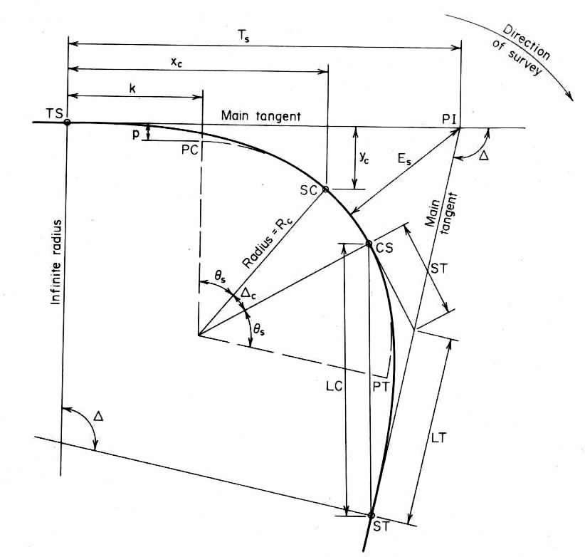
Fig. 198 Notaional system for transition spirals
|
In addition to the foregoing, there is a long tangent (LT), short tangent (ST), and lond cord (LC), as indicated with reespect to the departure sprial.
Place the origin of coordinates at the TS and the x axis on the main tangent.
Then: xsubc and ysubc = coordinates of SC;
k and p = abscissa and ordinate, respectively, of PC.
The coordinates of the SC and PC are useful as parameters in the calculation of
required distances. the distance p is termed the "throw or shift" of the curve;
it represents the displacement of the circular curve from the main tangent resulting from interposition of the spiral.
The basic angles are as follows:
Delta = angle between main tangents, or intersection angle;
DeltaC = angle between radii at SC and CS, or central angle of circular cureve;
PhataS = angle between radii of spiral at TS and SC, or central angle of entire spiral;
Dsubc = degree of curve of circular curve;
D = degree of curve at given point on spiral;
SigmS = deflection angle of SC from main tangent, with transit at TS;
Sigma = deflection angle of a given point on spiral from main tangent, with transit at TS.
Consider that a vehicle starts at the TS and traverses the approach spiral at constant speed. The degree of curve, which is zero at the TS, increases at a
uniform rate to become DsubC at the SC.
The basic equations are as follows:
Eq.(131);
PhataS = Lsubs * Dsubc / 200 = Lsubs / 2RsubC
Eq.(132)
xsubc = Lsubs (1 - PhataS sqr / 10)
Eq.(133)
ysubc = Lsubs ( PhataS / 3 - PhataS cubed / 42)
Eq.(134)
k = xsubc - Rsubc sin PhataS
Eq.(136)
SigmS = Lsubs / 6Rsubc = PhataS / 3
Eq.(137)
y = (L / Lsubs) cubed * ysubc
Eq.(138)
sigma = (L / Lsubs) sqr * SigmS
Eq.(139)
Tsubs = (Rsubc + p) tan 1/2 Delta + k
Eq.(140)
Esubs = (Rsubc + p)(sec 1/2 Delta - 1) + p
Eq.(141)
LT = xsubc - ysubc cot PhataS
Eq.(142)
ST = ysubc csc PhataS
Even though several of the foregoing equations are actually approximations, their use is valid when the value of Dsubc is relatively small.
Calculating the basic values:
|
Delta = 52 degrees 48 mins.;
Lsubs = 350ft;
Dsubc = 6 degrees;
PhataS = Lsubs * Dsubc / 200 = 350 (6) / 200 = 10.5 degrees = 10 degrees 30mins;
PhataS = 10.5 (0.017453) = 0.18326 rad;
DeltaC = 52 degrees 48 mins - 2 (10 degrees 30 mins) = 31 degrees 48 mins;
Dsubc = 6 (0.017453) = 0.10472 rad;
Rsubc = 100 / (Dsubc = 954.93ft;
xsubc = 350 (1 - 0.18326 spr / 10) = 348.83ft;
ysubc = 350 (0.18326 / 3 - 0.18326 sqr / 42) = 21.33ft;
k = 348.83 - 954.93 sin 10 degree 30 mins = 174.80ft;
p = 21.33 - 954.93 (1 - cos 10 degree 30 mins = 5.34ft.
Locate the TS and SC:
Thus, Tsubs = (954.93 + 5.34) tan 26 degrees 24 mins + 174.80 = 651.47;
station of TS = (34 + 93.81) - (6 + 51.47) = 28 + 42.34;
station of SC = (28 + 42.34) + (3 + 50.00) = 31 + 92.34.
Calculate the deflection angles:
Thus SigmS = 10 degrees 30 mins / 3 = 3 degrees 30 mins = 3.5 degrees.
Apply Eq.(138) to find the deflection angles at the intermediate stations.
For Example; for point 7, Sigma = 0.7 sqr (3.5 degrees) = 1.715 degrees = 1 degree 24.9 mins
Record the results in Table 13. The chord lengths beweeen successive stations differ
from the corresponding arc lengths by negligible amounts, and therefore each chord
length may be taken as 35.00ft.
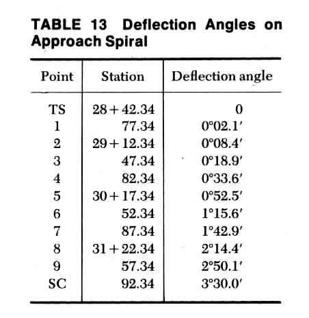
Table 13 Deflection Angles on Approach Spril
|
Compute the LT, ST, and Esubs:
Thus, LT = 348.83 - 21.33 cot 10 degree 30 mins = 233.75ft;
ST = 21.33 csc 10 degrees 30 mins = 117.04ft;
Esubs = (954.93 + 5.34)(sec 26 degrees 24 mins - 1) + 5.34 = 117.14ft
Verify the last three calculations by substitution:
Thus, (ST + Rsubc tan 1/2 DeltaC) / cos 1/2 Delta = (Tsubs - LT) / cos 1/2 Deltac =
1/2 Deltac = [ Esubs - Rsubc (sec 1/2 Deltac - 1)] / sin PhataS
Eq(143)